One-Step Actor-Critic Algorithm
Monte Carlo implementations like those of REINFORCE and baseline do not bootstrap, so they are slow to learn. Temporal difference solutions do bootstrap and can be incorporated into policy gradient algorithms in the same way that n-Step algorithms use it. The addition of n-Step expected returns to the REINFORCE with baseline algorithm yeilds an n-Step actor-critic.
I’m not a huge fan of the actor-critic terminology, because it obfuscates the fact that it is simply REINFORCE with a baseline, where the expected return is implemented as n-Step returns. That’s it.
I’ll implement that below and you’ll be suprised how similar the algorithm is. However, this time I’m going to use tile coding to encode the continous state space, to get a better baseline estimate.
A note on usage
Note that this notebook might not work on your machine because simple_rl forces TkAgg on some machines. See https://github.com/david-abel/simple_rl/issues/40
Also, Pygame is notoriously picky and expects loads of compiler/system related libraries.
I managed to get this working on the following notebook: docker run -it -p 8888:8888 jupyter/scipy-notebook:54462805efcb
This code is untested on any other notebook.
TODO: migrate away from simple rl and pygame. TODO: Create dedicated q-learning and sarsa notebooks.
!pip install pygame==1.9.6 pandas==1.0.5 matplotlib==3.2.1 gym==0.17.3 > /dev/null
!pip install --upgrade git+git://github.com/david-abel/simple_rl.git@77c0d6b910efbe8bdd5f4f87337c5bc4aed0d79c > /dev/null
import matplotlib
matplotlib.use("agg", force=True)
Running command git clone -q git://github.com/david-abel/simple_rl.git /tmp/pip-req-build-hmg3ra74
Setup and Previous Agents
This is the previous REINFORCE with baseline implementation. Take a look at the previous notebook if you are interested.
import gym
import random
import numpy as np
from simple_rl.tasks import GymMDP


# Gym MDP
gym_mdp = GymMDP(env_name="CartPole-v1", render=False)
num_feats = gym_mdp.get_num_state_feats()

GLOBAL_SEED = 0
random.seed(GLOBAL_SEED)
np.random.seed(GLOBAL_SEED)
gym_mdp.env.seed(GLOBAL_SEED)

from simple_rl.agents import PolicyGradientAgent

class LogisticPolicyAgent(PolicyGradientAgent):
    def __init__(self, actions, num_feats):
        self.α = 0.01
        self.γ = 0.99
        self.num_feats = num_feats
        PolicyGradientAgent.__init__(
            self, name="logistic_policy_gradient", actions=actions
        )
        self.reset()

    @staticmethod
    def logistic(x):
        return 1 / (1 + np.exp(-x))

    @staticmethod
    def π(θ, s):
        π = LogisticPolicyAgent.logistic(np.dot(θ.T, s))
        return np.array([π, 1 - π])

    @staticmethod
    def Δ(θ, s):
        π = LogisticPolicyAgent.logistic(np.dot(θ.T, s))
        return np.array([s - s * π, -s * π])

    def act(self, state, reward):
        if self.previous_pair is not None:
            self.episode_history.append(Step(self.previous_pair, reward))
        π = LogisticPolicyAgent.π(self.θ, state)
        action = np.random.choice((0, 1), p=π)
        self.previous_pair = Pair(state.data, action)
        return action

    def reset(self):
        self.θ = np.zeros(self.num_feats)
        self.end_of_episode()
        PolicyGradientAgent.reset(self)

    def end_of_episode(self):
        T = len(getattr(self, "episode_history", []))
        G = 0
        grad_buf = []
        for t in reversed(range(T)):
            G = G * self.γ + self.episode_history[t].reward
            grad = LogisticPolicyAgent.Δ(self.θ, self.episode_history[t].pair.state)[
                self.episode_history[t].pair.action
            ]
            self.θ += self.α * np.power(self.γ, t) * grad * G
            grad_buf.append(np.power(self.γ, t) * grad * G)
        reinforce_gradient_buffer.append(
            [np.mean(np.abs(grad_buf)), np.std(grad_buf)])
        self.episode_history = []
        self.previous_pair = None
        PolicyGradientAgent.end_of_episode(self)

class LogisticPolicyAgentWithBaseline(PolicyGradientAgent):
    def __init__(self, actions, num_feats, α_θ=0.01, prefix=""):
        self.α_θ = α_θ
        self.α_w = 0.1
        self.γ = 0.99
        self.num_feats = num_feats
        PolicyGradientAgent.__init__(
            self, name=prefix + "logistic_policy_gradient_with_baseline", actions=actions
        )
        self.reset()

    def act(self, state, reward):
        if self.previous_pair is not None:
            self.episode_history.append(Step(self.previous_pair, reward))
        π = LogisticPolicyAgent.π(self.θ, state)
        action = np.random.choice((0, 1), p=π)
        self.previous_pair = Pair(state.data, action)
        self.t += 1
        return action

    def reset(self):
        self.θ = np.zeros(self.num_feats)
        self.w = 0
        self.end_of_episode()
        PolicyGradientAgent.reset(self)

    def end_of_episode(self):
        self.t = 0
        T = len(getattr(self, "episode_history", []))
        G = 0
        grad_buf = []
        for t in reversed(range(T)):
            G = G * self.γ + self.episode_history[t].reward
            δ = G - self.w
            global_buffer.append(
                np.concatenate(
                    [self.episode_history[t].pair.state, np.array([G])])
            )
            self.w += self.α_w * δ
            Δπ = LogisticPolicyAgent.Δ(self.θ, self.episode_history[t].pair.state)[
                self.episode_history[t].pair.action
            ]
            self.θ += self.α_θ * np.power(self.γ, t) * δ * Δπ
            grad_buf.append(np.power(self.γ, t) * δ * Δπ)
        baseline_gradient_buffer.append(
            [np.mean(np.abs(grad_buf)), np.std(grad_buf)])
        self.episode_history = []
        self.previous_pair = None
        PolicyGradientAgent.end_of_episode(self)
Warning: Tensorflow not installed.
Tile Coding
Tile coding attemps to split the feature space into discrete bins, where you set the bin to 1 if the value is contained within that bin. If you overlap the bin boundaries, you end up with quite an accurate representation of a continuous feature in discrete form.
TODO: In depth article example about tile coding.
# Taken from https://github.com/MeepMoop/tilecoding
class TileCoder:
    def __init__(
        self,
        tiles_per_dim,
        value_limits,
        tilings,
        offset=lambda n: 2 * np.arange(n) + 1,
    ):
        tiling_dims = np.array(np.ceil(tiles_per_dim), dtype=np.int) + 1
        self._offsets = (
            offset(len(tiles_per_dim))
            * np.repeat([np.arange(tilings)], len(tiles_per_dim), 0).T
            / float(tilings)
            % 1
        )
        self._limits = np.array(value_limits)
        self._norm_dims = np.array(tiles_per_dim) / (
            self._limits[:, 1] - self._limits[:, 0]
        )
        self._tile_base_ind = np.prod(tiling_dims) * np.arange(tilings)
        self._hash_vec = np.array(
            [np.prod(tiling_dims[0:i]) for i in range(len(tiles_per_dim))]
        )
        self._n_tiles = tilings * np.prod(tiling_dims)

    def __getitem__(self, x):
        off_coords = (
            (x - self._limits[:, 0]) * self._norm_dims + self._offsets
        ).astype(int)
        return self._tile_base_ind + np.dot(off_coords, self._hash_vec)

    @property
    def n_tiles(self):
        return self._n_tiles
n-Step Actor-Critic Algorithm
The major addition in this implementation is the use of Tile Coding for the baseline estimate. This improves performance over the previous rolling average method. In addition you will also notice the use of the next state to predict the 1-step expected return. There are no other differences.
class OneStepActorCritic(PolicyGradientAgent):
    @staticmethod
    def v(w, S):
        return np.dot(w.T, S)

    @staticmethod
    def Δv(w, S):
        return S

    def augment(self, S):
        S = S[2:]
        a = np.zeros(self.T.n_tiles)
        a[self.T[S]] = 1
        return a

    def __init__(self, actions, num_feats, α_θ=0.01, α_w=0.1, prefix=""):
        self.α_θ = α_θ
        self.α_w = α_w
        self.γ = 0.99
        self.num_feats = num_feats
        # tile coder tiling dimensions, value limits, number of tilings
        tiles_per_dim = [10] * num_feats
        lims = [(-0.72, 0.72), (-5, 5)]
        tilings = 5
        self.T = TileCoder(tiles_per_dim, lims, tilings)
        print(self.T.n_tiles)
        PolicyGradientAgent.__init__(
            self, name=prefix + "one_step_actor_critic", actions=actions
        )
        self.reset()

    def update(self, state, action, reward, next_state, terminal: bool):
        raw_state = state.copy()
        state = self.augment(state)
        next_state = self.augment(next_state)

        v = self.v(self.w, state)
        if terminal:
            δ = reward + self.γ * 0 - v
        else:
            δ = reward + self.γ * self.v(self.w, next_state) - v
        self.w += self.α_w * δ * self.Δv(self.w, state)
        self.θ += (
            self.α_θ * self.I * δ *
            LogisticPolicyAgent.Δ(self.θ, raw_state)[action]
        )
        self.I *= self.γ

    def act(self, state, reward):
        if self.previous_pair is not None:
            self.update(
                self.previous_pair.state,
                self.previous_pair.action,
                reward,
                state.data,
                state.is_terminal(),
            )
        π = LogisticPolicyAgent.π(self.θ, state)
        action = np.random.choice((0, 1), p=π)
        self.previous_pair = Pair(state.data, action)
        self.t += 1
        return action

    def reset(self):
        self.θ = np.zeros(4)
        self.w = np.zeros(self.T.n_tiles)
        self.end_of_episode()
        PolicyGradientAgent.reset(self)

    def end_of_episode(self):
        # print(np.mean(self.w), np.std(self.w), np.min(self.w), np.max(self.w), np.count_nonzero(self.w) / self.T.n_tiles)
        self.I = 1
        self.t = 0
        self.previous_pair = None
        PolicyGradientAgent.end_of_episode(self)
Training the Agent
Now I’m ready to run the experiment to train the agents. I reduce the number of instances to 1 now to save time, since I’m trying to run 4 separate algorithms. If you increase the number of repetitions this will smooth out the results.
from simple_rl.run_experiments import run_agents_on_mdp
from collections import namedtuple

Step = namedtuple("Step", ["pair", "reward"])
Pair = namedtuple("Pair", ["state", "action"])

global_buffer = []
baseline_gradient_buffer = []
REINFORCE_baseline = LogisticPolicyAgentWithBaseline(
    gym_mdp.get_actions(), num_feats
)
run_agents_on_mdp(
    [REINFORCE_baseline],
    gym_mdp,
    instances=1,
    episodes=500,
    steps=1000,
    open_plot=False,
    verbose=False,
    cumulative_plot=False,
)
np.savetxt("state_reward_REINFORCE_baseline.txt", np.array(global_buffer))
np.savetxt("gradient_REINFORCE_baseline.txt",
            np.array(baseline_gradient_buffer))

TDAC_slow = OneStepActorCritic(
    gym_mdp.get_actions(), 2, α_θ=0.1, α_w=0.01, prefix="slow_weight_")
TDAC_fast = OneStepActorCritic(
    gym_mdp.get_actions(), 2, α_θ=0.1, α_w=0.1, prefix="fast_weight_")
TDAC_super_fast = OneStepActorCritic(
    gym_mdp.get_actions(), 2, α_θ=0.1, α_w=0.5, prefix="super_fast_weight_")
run_agents_on_mdp(
    [TDAC_slow, TDAC_fast, TDAC_super_fast],
    gym_mdp,
    instances=1,
    episodes=500,
    steps=500,
    open_plot=False,
    verbose=False,
    cumulative_plot=False,
)
Running experiment:
(MDP)
    gym-CartPole-v1
(Agents)
    logistic_policy_gradient_with_baseline,0
(Params)
    instances : 1
    episodes : 500
    steps : 1000
    track_disc_reward : False

logistic_policy_gradient_with_baseline is learning.
  Instance 1 of 1.
/opt/conda/lib/python3.7/site-packages/numpy/core/fromnumeric.py:3335: RuntimeWarning: Mean of empty slice.
  out=out, **kwargs)
/opt/conda/lib/python3.7/site-packages/numpy/core/_methods.py:161: RuntimeWarning: invalid value encountered in double_scalars
  ret = ret.dtype.type(ret / rcount)
/opt/conda/lib/python3.7/site-packages/numpy/core/_methods.py:217: RuntimeWarning: Degrees of freedom <= 0 for slice
  keepdims=keepdims)
/opt/conda/lib/python3.7/site-packages/numpy/core/_methods.py:186: RuntimeWarning: invalid value encountered in true_divide
  arrmean, rcount, out=arrmean, casting='unsafe', subok=False)
/opt/conda/lib/python3.7/site-packages/numpy/core/_methods.py:209: RuntimeWarning: invalid value encountered in double_scalars
  ret = ret.dtype.type(ret / rcount)


--- TIMES ---
logistic_policy_gradient_with_baseline agent took 71.56 seconds.
-------------

    logistic_policy_gradient_with_baseline: 500.0 (conf_interv: 0.0 )
605
605
605
Running experiment:
(MDP)
    gym-CartPole-v1
(Agents)
    slow_weight_one_step_actor_critic,0
    fast_weight_one_step_actor_critic,1
    super_fast_weight_one_step_actor_critic,2
(Params)
    instances : 1
    episodes : 500
    steps : 500
    track_disc_reward : False

slow_weight_one_step_actor_critic is learning.
  Instance 1 of 1.

fast_weight_one_step_actor_critic is learning.
  Instance 1 of 1.

super_fast_weight_one_step_actor_critic is learning.
  Instance 1 of 1.


--- TIMES ---
slow_weight_one_step_actor_critic agent took 85.71 seconds.
fast_weight_one_step_actor_critic agent took 113.61 seconds.
super_fast_weight_one_step_actor_critic agent took 117.25 seconds.
-------------

    slow_weight_one_step_actor_critic: 500.0 (conf_interv: 0.0 )
    fast_weight_one_step_actor_critic: 500.0 (conf_interv: 0.0 )
    super_fast_weight_one_step_actor_critic: 500.0 (conf_interv: 0.0 )
Plotting the Results
The following will read from the saved results.
%matplotlib inline
import matplotlib
import matplotlib.pyplot as plt
import numpy as np
import pandas as pd
def plot(experiment_name, data_files, cutoff=None):
fig, ax = plt.subplots(nrows=1, ncols=1)
for j, (name, data_file) in enumerate(data_files):
df = pd.read_csv(data_file, header=None).transpose()
if cutoff:
df = df.truncate(after=cutoff)
x = df.index.values
y = df.values
if len(y.shape) > 1:
y = y.mean(axis=1)
ax.yaxis.major.formatter._useMathText = True
ax.plot(x,
y,
label=name)
ax.set_xlabel('Epoch')
ax.set_ylabel('Average Reward (1 run)')
ax.legend(loc='lower right')
plt.show()
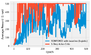
data_files = [
("REINFORCE with baseline (logistic)", "results/gym-CartPole-v1/logistic_policy_gradient_with_baseline.csv"),
("1-Step Actor-Critic", "results/gym-CartPole-v1/fast_weight_one_step_actor_critic.csv"),
]
plot("reinforce_reward_plot", data_files, cutoff=500)
data_files = [
    ("1-Step Actor-Critic (α_w = 0.01)", "results/gym-CartPole-v1/slow_weight_one_step_actor_critic.csv"),
    ("1-Step Actor-Critic (α_w = 0.1)", "results/gym-CartPole-v1/fast_weight_one_step_actor_critic.csv"),
    ("1-Step Actor-Critic (α_w = 0.5)", "results/gym-CartPole-v1/super_fast_weight_one_step_actor_critic.csv"),
]
plot("reinforce_reward_plot", data_files, cutoff=500)
Discussion
Algorithms that can bootstrap, or in other words, algorithms that can learn from the get-go, learn faster than those that have to wait until an episode is over. n-step algorithms do this and the first plots demonstrates the increase in performance. The plot is a little noisy due to no averaging.
The second image shows the difference between different learning rate parameters. The fastest (0.5) is very unstable. Sometimes it learns, other times it doesn’t, because the policy is changing on each step. The slow (0.01) has a similar performance to the Monte Carlo methods. The learning rate in the middle (0.1) learns fast and is about as stable as the other algorithms. This demonstrates how you must tune your hyperparameters to your specific problem.