REINFORCE: Monte Carlo Policy Gradient Methods
Policy gradient methods work by first choosing actions directly from a parameterized model, then secondly updating the weights of the model to nudge the next predictions towards higher expected returns.
REINFORCE achieves this by collecting a full trajectory then updating the policy weights in a Monte Carlo-style.
To demonstrate this I will implement REINFORCE in simple_rl using a logistic policy model.
A note on usage
Note that this notebook might not work on your machine because simple_rl forces TkAgg on some machines. See https://github.com/david-abel/simple_rl/issues/40
Also, Pygame is notoriously picky and expects loads of compiler/system related libraries.
I managed to get this working on the following notebook: docker run -it -p 8888:8888 jupyter/scipy-notebook:54462805efcb
This code is untested on any other notebook.
TODO: migrate away from simple rl and pygame. TODO: Create dedicated q-learning and sarsa notebooks.
!pip install pygame==1.9.6 pandas==1.0.5 matplotlib==3.2.1 gym==0.17.3 > /dev/null
!pip install --upgrade git+git://github.com/david-abel/simple_rl.git@77c0d6b910efbe8bdd5f4f87337c5bc4aed0d79c > /dev/null
import matplotlib
matplotlib.use("agg", force=True)
Running command git clone -q git://github.com/david-abel/simple_rl.git /tmp/pip-req-build-gw4_9f_w
Setup and the Environment
For this experiment I will use the cartpole environment. Then I set the seeds to produce consistent results.
import gym
import random
import numpy as np
from simple_rl.tasks import GymMDP


# Gym MDP
gym_mdp = GymMDP(env_name="CartPole-v1", render=False)
num_feats = gym_mdp.get_num_state_feats()
Warning: Tensorflow not installed.
GLOBAL_SEED = 0
random.seed(GLOBAL_SEED)
np.random.seed(GLOBAL_SEED)
gym_mdp.env.seed(GLOBAL_SEED)
[0]
REINFORCE Agent
The code below defines the REINFORCE agent. The key to this implementation is that I have manually differentiated the logistic function so the gradient can be calculated directly. In reality you would probably use an automatic differentiation framework, or use a framework that provides the gradients for you.
Once you have the gradient, then all you need to do is use the policy gradient update rule to nudge the parameters towards areas of higher return.
from simple_rl.agents import PolicyGradientAgent

class LogisticPolicyAgent(PolicyGradientAgent):
    def __init__(self, actions, num_feats):
        self.α = 0.01
        self.γ = 0.99
        self.num_feats = num_feats
        PolicyGradientAgent.__init__(
            self, name="logistic_policy_gradient", actions=actions
        )
        self.reset()

    @staticmethod
    def logistic(x):
        return 1 / (1 + np.exp(-x))

    @staticmethod
    def π(θ, s):
        π = LogisticPolicyAgent.logistic(np.dot(θ.T, s))
        return np.array([π, 1 - π])

    @staticmethod
    def Δ(θ, s):
        π = LogisticPolicyAgent.logistic(np.dot(θ.T, s))
        return np.array([s - s * π, -s * π])

    def act(self, state, reward):
        if self.previous_pair is not None:
            self.episode_history.append(Step(self.previous_pair, reward))
        π = LogisticPolicyAgent.π(self.θ, state)
        action = np.random.choice((0, 1), p=π)
        self.previous_pair = Pair(state.data, action)
        return action

    def reset(self):
        self.θ = np.zeros(self.num_feats)
        self.end_of_episode()
        PolicyGradientAgent.reset(self)

    def end_of_episode(self):
        T = len(getattr(self, "episode_history", []))
        G = 0
        grad_buf = []
        for t in reversed(range(T)):
            G = G * self.γ + self.episode_history[t].reward
            grad = LogisticPolicyAgent.Δ(self.θ, self.episode_history[t].pair.state)[
                self.episode_history[t].pair.action
            ]
            self.θ += self.α * np.power(self.γ, t) * grad * G
            grad_buf.append(np.power(self.γ, t) * grad * G)
        reinforce_gradient_buffer.append(
            [np.mean(np.abs(grad_buf)), np.std(grad_buf)])
        self.episode_history = []
        self.previous_pair = None
        PolicyGradientAgent.end_of_episode(self)
Training the Agent
Now I’m ready to run the experiment to train the agent. You might want to play around with the instances parameter, which controls the number of repeats to average over.
from simple_rl.run_experiments import run_agents_on_mdp
from collections import namedtuple

Step = namedtuple("Step", ["pair", "reward"])
Pair = namedtuple("Pair", ["state", "action"])

reinforce_gradient_buffer = []
REINFORCE = LogisticPolicyAgent(gym_mdp.get_actions(), num_feats)
run_agents_on_mdp(
    [REINFORCE],
    gym_mdp,
    instances=2,
    episodes=500,
    steps=1000,
    open_plot=False,
    verbose=False,
    cumulative_plot=False,
)
np.savetxt("gradient_REINFORCE.txt", np.array(reinforce_gradient_buffer))
Running experiment:
(MDP)
    gym-CartPole-v1
(Agents)
    logistic_policy_gradient,0
(Params)
    instances : 2
    episodes : 500
    steps : 1000
    track_disc_reward : False

logistic_policy_gradient is learning.
  Instance 1 of 2.
/opt/conda/lib/python3.7/site-packages/numpy/core/fromnumeric.py:3335: RuntimeWarning: Mean of empty slice.
  out=out, **kwargs)
/opt/conda/lib/python3.7/site-packages/numpy/core/_methods.py:161: RuntimeWarning: invalid value encountered in double_scalars
  ret = ret.dtype.type(ret / rcount)
/opt/conda/lib/python3.7/site-packages/numpy/core/_methods.py:217: RuntimeWarning: Degrees of freedom <= 0 for slice
  keepdims=keepdims)
/opt/conda/lib/python3.7/site-packages/numpy/core/_methods.py:186: RuntimeWarning: invalid value encountered in true_divide
  arrmean, rcount, out=arrmean, casting='unsafe', subok=False)
/opt/conda/lib/python3.7/site-packages/numpy/core/_methods.py:209: RuntimeWarning: invalid value encountered in double_scalars
  ret = ret.dtype.type(ret / rcount)
  Instance 2 of 2.


--- TIMES ---
logistic_policy_gradient agent took 146.32 seconds.
-------------

    logistic_policy_gradient: 236.5 (conf_interv: 78.31 )
Plotting the Results
The following will read from the saved results.
%matplotlib inline
import matplotlib
import matplotlib.pyplot as plt
from matplotlib.ticker import ScalarFormatter, AutoMinorLocator
import matplotlib as mpl
import json
import os
import numpy as np
import pandas as pd
from pathlib import Path
from glob import glob
import subprocess
def plot(experiment_name, data_files, cutoff=None):
fig, ax = plt.subplots(nrows=1, ncols=1)
for j, (name, data_file) in enumerate(data_files):
df = pd.read_csv(data_file, header=None).transpose()
if cutoff:
df = df.truncate(after=cutoff)
x = df.index.values
y = df.values
if len(y.shape) > 1:
y = y.mean(axis=1)
ax.plot(x,
y,
label=name)
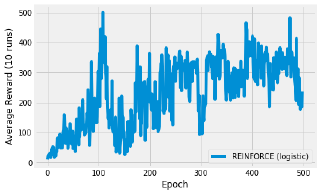
ax.set_xlabel('Epoch')
ax.set_ylabel('Average Reward (10 runs)')
ax.legend(loc='lower right')
plt.show()
data_files = [
("REINFORCE (logistic)", "results/gym-CartPole-v1/logistic_policy_gradient.csv"),
]
plot("reinforce_reward_plot", data_files, cutoff=500)
Discussion
The image above shows the result of plotting the average reward over 500 episodes. The specific curve will depend on your seed and the number of repetitions to average over.
The thing to take away from this experiment is the sheer simplicity of what is going on here. I have defined a very simple model and manually derived the gradient. The environment has 4 continuous features so I need a 4-parameter model. To find an optimal policy, you just need to nudge the gradients towards higher returns. That’s it!
This means that policy gradient methods work really well with continuous state spaces, where value-based methods would struggle, due to the required discretisation.