n-Step Methods
Another fundamental algorithm is the use of n-Step returns, rather than single step returns in the basic Q-learning or SARSA implementations. Rather than just looking one step into the future and estimating the return, you can look several steps. This is implemented in a backwards fashion, where you should travel first then updates the states you have visited. But it works really well.
This notebook builds upon the Q-learning and SARSA notebooks, so I recommend you see them first.
A note on usage
Note that this notebook might not work on your machine because simple_rl forces TkAgg on some machines. See https://github.com/david-abel/simple_rl/issues/40
Also, Pygame is notoriously picky and expects loads of compiler/system related libraries.
I managed to get this working on the following notebook:
docker run -it -p 8888:8888 jupyter/scipy-notebook:54462805efcb
This code is untested on any other notebook.
TODO: migrate away from simple rl and pygame. TODO: Create dedicated q-learning and sarsa notebooks.
!pip install pygame==1.9.6 pandas==1.0.5 matplotlib==3.2.1 > /dev/null
!pip install --upgrade git+git://github.com/david-abel/simple_rl.git@77c0d6b910efbe8bdd5f4f87337c5bc4aed0d79c > /dev/null
import matplotlib
matplotlib.use("agg", force=True)
Running command git clone -q git://github.com/david-abel/simple_rl.git /tmp/pip-req-build-dgz_vdaj
n-Step SARSA Agent
simple_rl doesn’t come with an n-Step SARSA implementation so I must create one first. The code is below. Again, most of the complexity is due to the library abstractions. The most important code is in the update function.
import numpy as np
import sys
from collections import defaultdict
from simple_rl.agents import Agent, QLearningAgent


class nStepSARSAAgent(QLearningAgent):
    def __init__(self, actions, n, name="n-Step SARSA",
                 alpha=0.1, gamma=0.99, epsilon=0.1, explore="uniform", anneal=False):
        self.T = sys.maxsize
        self.stored_rewards = []
        self.stored_states = []
        self.stored_actions = []
        self.n = n
        QLearningAgent.__init__(
            self,
            actions=list(actions),
            name=name,
            alpha=alpha,
            gamma=gamma,
            epsilon=epsilon,
            explore=explore,
            anneal=anneal)

    def policy(self, state):
        return self.get_max_q_action(state)

    def act(self, state, reward, learning=True):
        action = self.update(reward, state)
        return action

    def update(self, rt1, st1):
        if len(self.stored_states) == 0:
            action = self.epsilon_greedy_q_policy(st1)
            self.stored_actions.append(action)
            self.stored_states.append(st1)
            self.stored_rewards.append(rt1)
            return action

        if self.step_number < self.T:
            # Observe and store the next reward R_{t+1} and next state
            # S_{t+1}
            self.stored_rewards.append(rt1)
            self.stored_states.append(st1)

            # if s_{t+1} terminal
            if st1.is_terminal():
                self.T = self.step_number + 1
            else:
                action = self.epsilon_greedy_q_policy(st1)
                self.stored_actions.append(action)

        self.tau = self.step_number - self.n + 1
        if self.tau >= 0:
            # G = sum(\gamma * R)
            start_index = self.tau + 1
            end_index = min(self.tau + self.n, self.T)
            G = 0
            for i in range(
                    start_index, end_index + 1):  # Because range is exclusive
                G += self.gamma**(i - self.tau - 1) * self.stored_rewards[i]

            if self.tau + self.n < self.T:
                G += self.gamma**self.n * \
                    self.q_func[self.stored_states[(
                        self.tau + self.n)]][self.stored_actions[(self.tau + self.n)]]
            s_tau = self.stored_states[self.tau]
            a_tau = self.stored_actions[self.tau]
            self.q_func[s_tau][a_tau] += self.alpha * \
                (G - self.q_func[s_tau][a_tau])
        # If at end repeat until tau == T - 1
        self.step_number += 1
        if self.step_number >= self.T and self.tau < self.T - 1:
            self.update(None, None)
        return self.stored_actions[-1]

    def end_of_episode(self):
        self.prev_state = None
        self.prev_action = None
        self.episode_number += 1
        self.T = sys.maxsize
        self.step_number = 0
        self.stored_rewards = []
        self.stored_states = []
        self.stored_actions = []

    def reset(self):
        self.prev_state = None
        self.prev_action = None
        self.step_number = 0
Warning: Tensorflow not installed.
Warning: OpenAI gym not installed.
Experiment
Similar to before, I run the agents on the CliffWorld inspired environment. First I setup the the global settings, instantite the environment, then I test the three algorithms and save the data.
If your not in a notebook you can use the visualize_policy function to visualise the policy. mdp.visualize_policy(ql_agent.policy) for example.
import pandas as pd
import numpy as np
from simple_rl.agents import DoubleQAgent, DelayedQAgent
from simple_rl.tasks import GridWorldMDP
from simple_rl.run_experiments import run_single_agent_on_mdp
from simple_rl.abstraction import AbstractionWrapper
from simple_rl.utils import chart_utils

np.random.seed(42)
visualise_double_q_learning = False
visualise_delayed_q_learning = False

instances = 10
n_episodes = 500
alpha = 0.1
epsilon = 0.1

# Setup MDP, Agents.
mdp = GridWorldMDP(
    width=10, height=4, init_loc=(1, 1), goal_locs=[(10, 1)],
    lava_locs=[(x, 1) for x in range(2, 10)], is_lava_terminal=True, gamma=1.0, walls=[], slip_prob=0.0, step_cost=1.0, lava_cost=100.0)

print("SARSA")
rewards = np.zeros((n_episodes, instances))
for instance in range(instances):
    ql_agent = nStepSARSAAgent(
        mdp.get_actions(),
        n=1,
        epsilon=epsilon,
        alpha=alpha)
    print("  Instance " + str(instance) + " of " + str(instances) + ".")
    terminal, num_steps, reward = run_single_agent_on_mdp(
        ql_agent, mdp, episodes=n_episodes, steps=100)
    rewards[:, instance] = reward
df = pd.DataFrame(rewards.mean(axis=1))
df.to_json("sarsa_cliff_rewards.json")

print("2-Step SARSA")
rewards = np.zeros((n_episodes, instances))
for instance in range(instances):
    ql_agent = nStepSARSAAgent(
        mdp.get_actions(),
        n=2,
        epsilon=epsilon,
        alpha=alpha)
    print("  Instance " + str(instance) + " of " + str(instances) + ".")
    terminal, num_steps, reward = run_single_agent_on_mdp(
        ql_agent, mdp, episodes=n_episodes, steps=100)
    rewards[:, instance] = reward
df = pd.DataFrame(rewards.mean(axis=1))
df.to_json("2_step_sarsa_cliff_rewards.json")

print("4-Step SARSA")
rewards = np.zeros((n_episodes, instances))
for instance in range(instances):
    ql_agent = nStepSARSAAgent(
        mdp.get_actions(),
        n=4,
        epsilon=epsilon,
        alpha=alpha)
    print("  Instance " + str(instance) + " of " + str(instances) + ".")
    terminal, num_steps, reward = run_single_agent_on_mdp(
        ql_agent, mdp, episodes=n_episodes, steps=100)
    rewards[:, instance] = reward
df = pd.DataFrame(rewards.mean(axis=1))
df.to_json("4_step_sarsa_cliff_rewards.json")
SARSA
  Instance 0 of 10.
  Instance 1 of 10.
  Instance 2 of 10.
  Instance 3 of 10.
  Instance 4 of 10.
  Instance 5 of 10.
  Instance 6 of 10.
  Instance 7 of 10.
  Instance 8 of 10.
  Instance 9 of 10.
2-Step SARSA
  Instance 0 of 10.
  Instance 1 of 10.
  Instance 2 of 10.
  Instance 3 of 10.
  Instance 4 of 10.
  Instance 5 of 10.
  Instance 6 of 10.
  Instance 7 of 10.
  Instance 8 of 10.
  Instance 9 of 10.
4-Step SARSA
  Instance 0 of 10.
  Instance 1 of 10.
  Instance 2 of 10.
  Instance 3 of 10.
  Instance 4 of 10.
  Instance 5 of 10.
  Instance 6 of 10.
  Instance 7 of 10.
  Instance 8 of 10.
  Instance 9 of 10.
Results
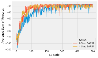
Below is the code to visualise the training of the three agents. There are a maximum of 100 steps, over 500 episodes, averaged over 10 repeats. Feel free to tinker with those settings.
The results show the differences between the three algorithms. In general, a higher value of n learns more quickly, with diminishing returns.
%matplotlib inline
import matplotlib.pyplot as plt
from matplotlib.ticker import ScalarFormatter, AutoMinorLocator
import json
import os
import numpy as np
import pandas as pd

data_files = [("SARSA", "sarsa_cliff_rewards.json"),
              ("2-Step SARSA", "2_step_sarsa_cliff_rewards.json"),
              ("4-Step SARSA", "4_step_sarsa_cliff_rewards.json")]
fig, ax = plt.subplots()
for j, (name, data_file) in enumerate(data_files):
    df = pd.read_json(data_file)
    x = range(len(df))
    y = df.sort_index().values
    ax.plot(x,
            y,
            linestyle='solid',
            linewidth=1,
            label=name)
ax.set_xlabel('Episode')
ax.set_ylabel('Averaged Sum of Rewards')
ax.legend(loc='lower right')
plt.show()